Results

Every figure and number on this page is produced by scripts/build_figures.py, which runs the package against the fetched dataset. Nothing here is hand-entered.

Sample

Period	2006-05-17 → 2026-09-11
Daily returns	4,988
EWMA decay (λ)	0.94
Confidence level	99% (α = 0.01)

Market data

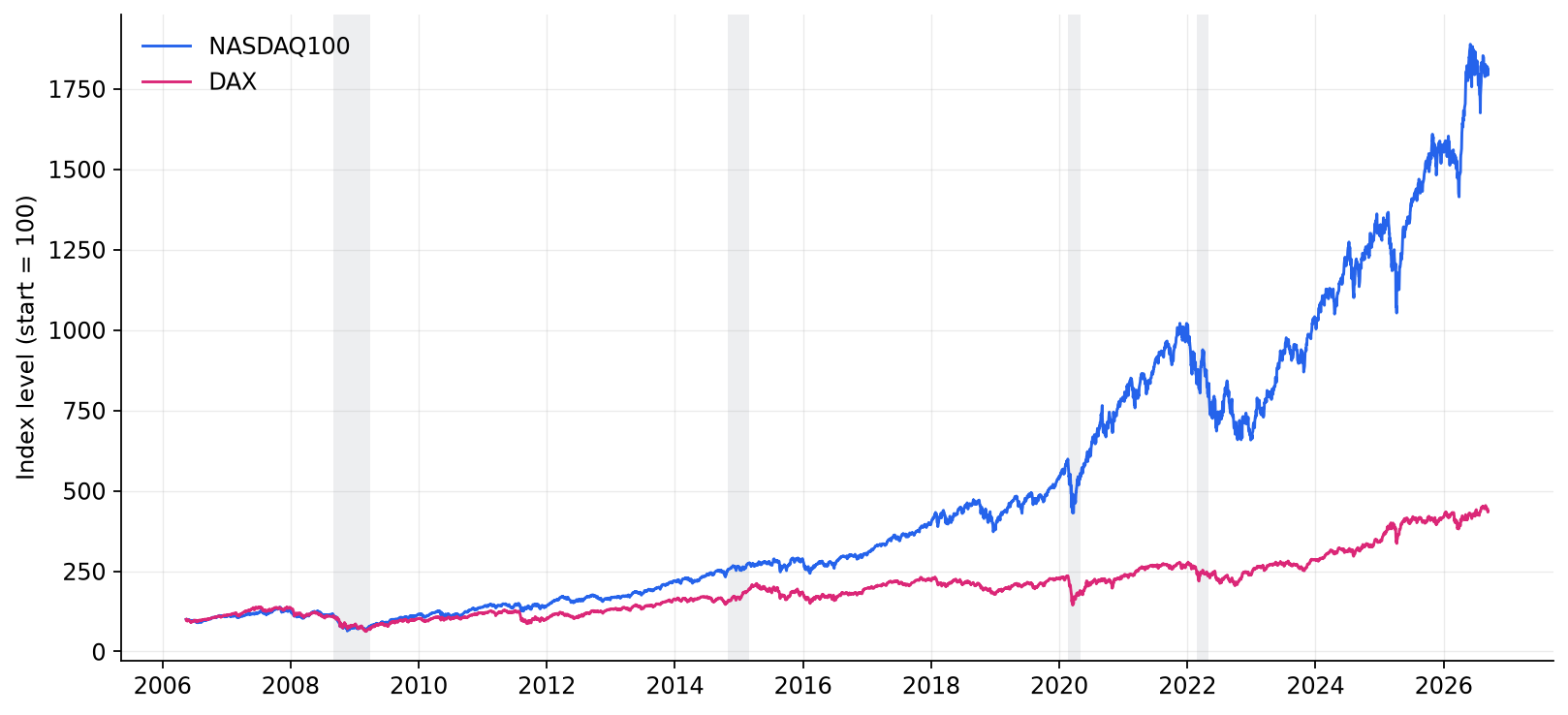
The NASDAQ 100 and DAX over the sample, rebased to 100. Shaded bands mark the four crisis windows.

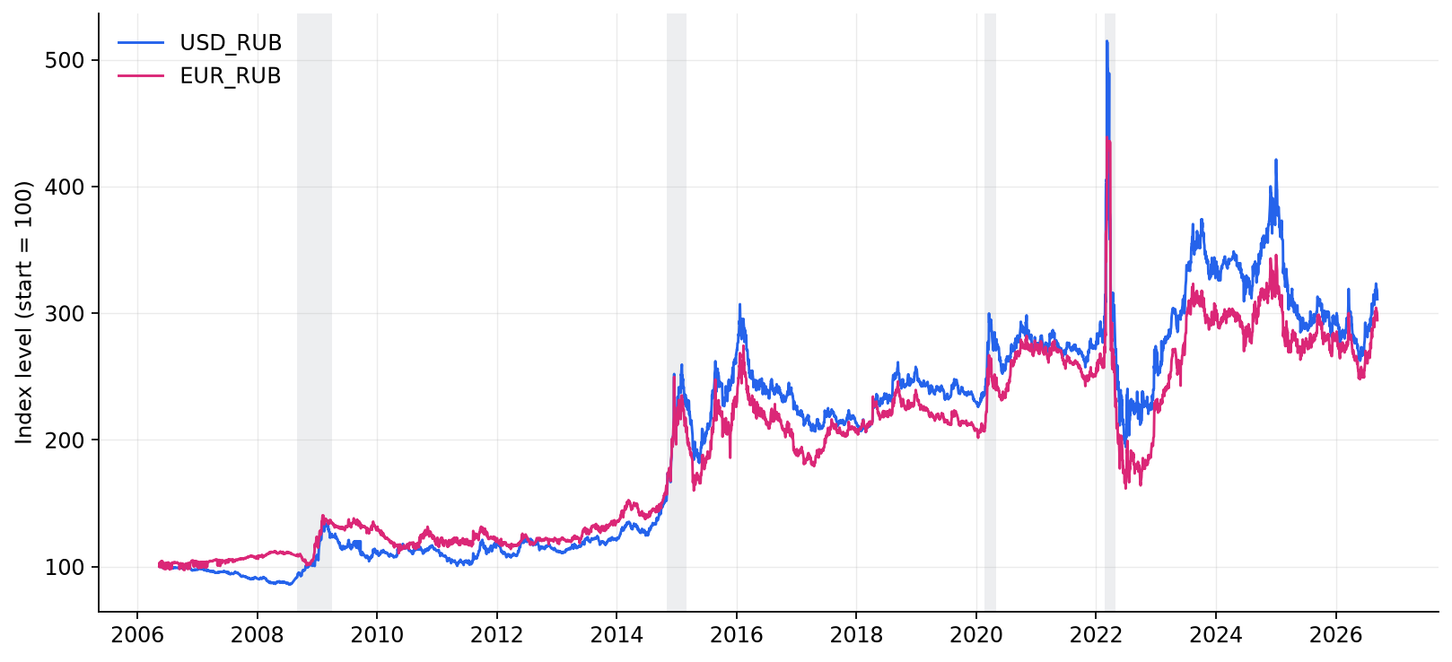
USD/RUB and EUR/RUB, rebased. Rising means a weakening ruble — note the step changes in late 2014 and early 2022, both of which persist rather than reverting.

Volatility

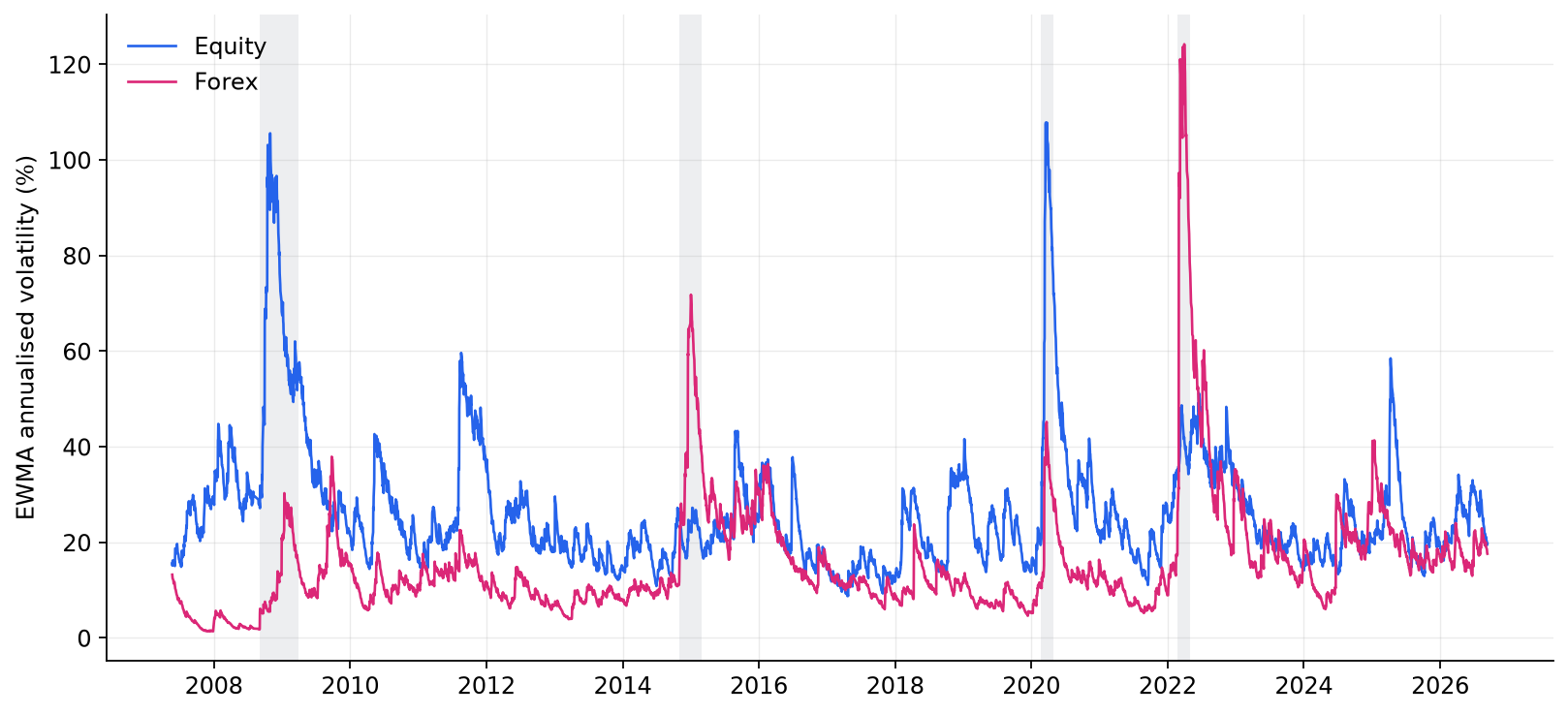
	Mean	Peak	Peak date
Equity	26.3%	107.8%	2020-03-19
Forex	15.8%	124.2%	2022-03-31

The headline result of the decomposition: the two components peak in different crises. Equity volatility spikes in 2008 and again in the COVID crash. Currency volatility barely reacts to either, then dominates in the 2014 ruble crisis and in 2022 — where it reaches a level equity volatility never touches anywhere in twenty years.

An investor looking only at aggregate portfolio volatility would see two spikes and conclude the portfolio has one risk driver that occasionally flares up. Splitting the series shows it has two, and they fire on different events.

Correlation

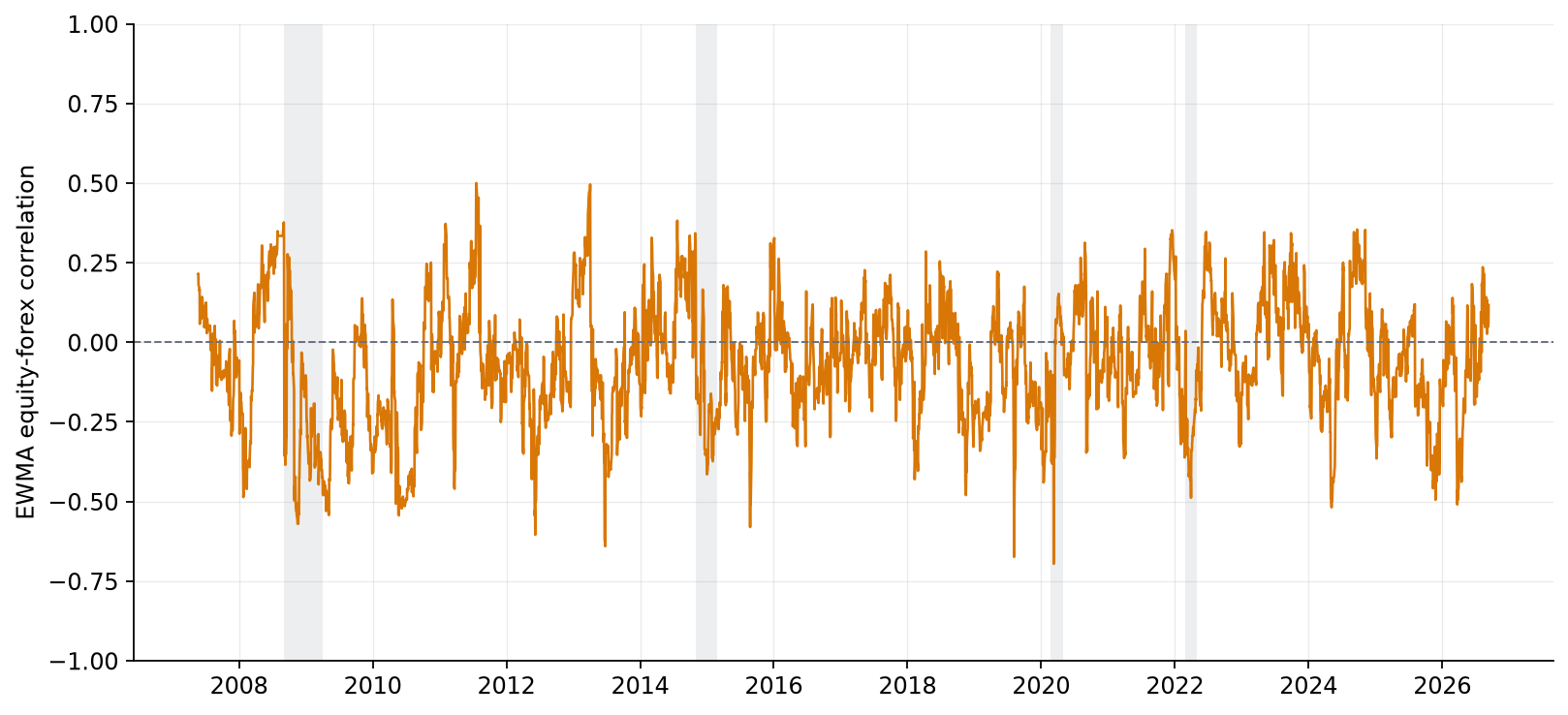
Mean	Minimum	Maximum
−0.064	−0.696	+0.500

The correlation between equity and currency returns swings across most of the available range. Averaging it to −0.06 and treating that as a constant would be badly misleading: the series spends long stretches meaningfully negative — where ruble depreciation cushions equity losses — and other stretches positive, where the two risks compound instead.

This is what the parametric VaR calculation is picking up when it uses a time-varying covariance matrix rather than a static one.

Return distribution

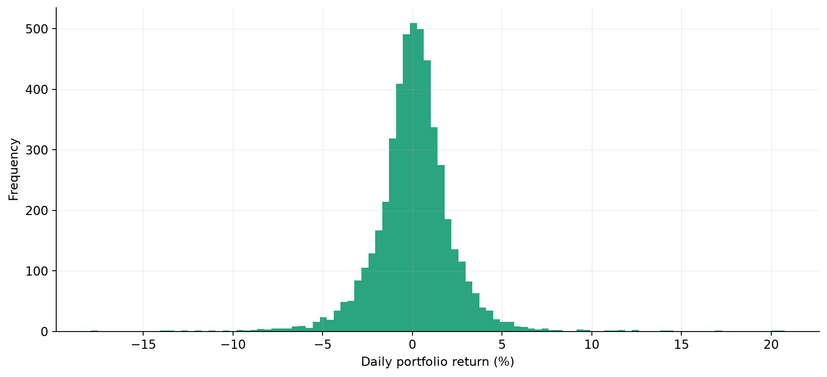
Broadly bell-shaped with visibly fat tails on both sides. The fat tails are precisely why the parametric and historical estimates below disagree: the normal distribution assumed by the former does not have enough mass out where the losses actually are.

Value-at-Risk

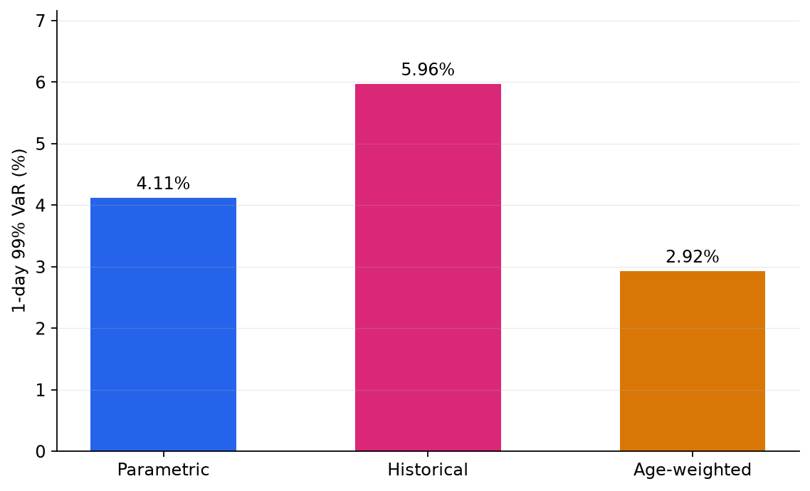
Method	1-day 99% VaR	10-day
Parametric	4.11%	13.00%
Historical	5.96%	18.85%
Age-weighted	2.92%	9.24%

Same portfolio, same data, same confidence level — and a spread of over three percentage points.

The ordering is informative. Historical is highest because the twenty-year sample contains crises far more severe than current conditions, and equal-weighting means 2008 counts as heavily as last month. Age-weighted is lowest because it discounts those distant crises in favour of the recent, calmer regime. Parametric sits between, driven by an EWMA covariance that reflects recent conditions but assumes a thin-tailed normal distribution.

Which is right?

None of them, individually. They answer slightly different questions — what has happened, what is happening lately, and what the model says — and the gap between them is itself the useful output: it measures how much the answer depends on that choice rather than on the data.

Does the model actually work?

Reporting a VaR number is easy; the harder question is whether it holds up. Because the EWMA estimates carry no look-ahead, the VaR for any given day is what the model would genuinely have forecast that morning — so it can be checked against what actually happened next.

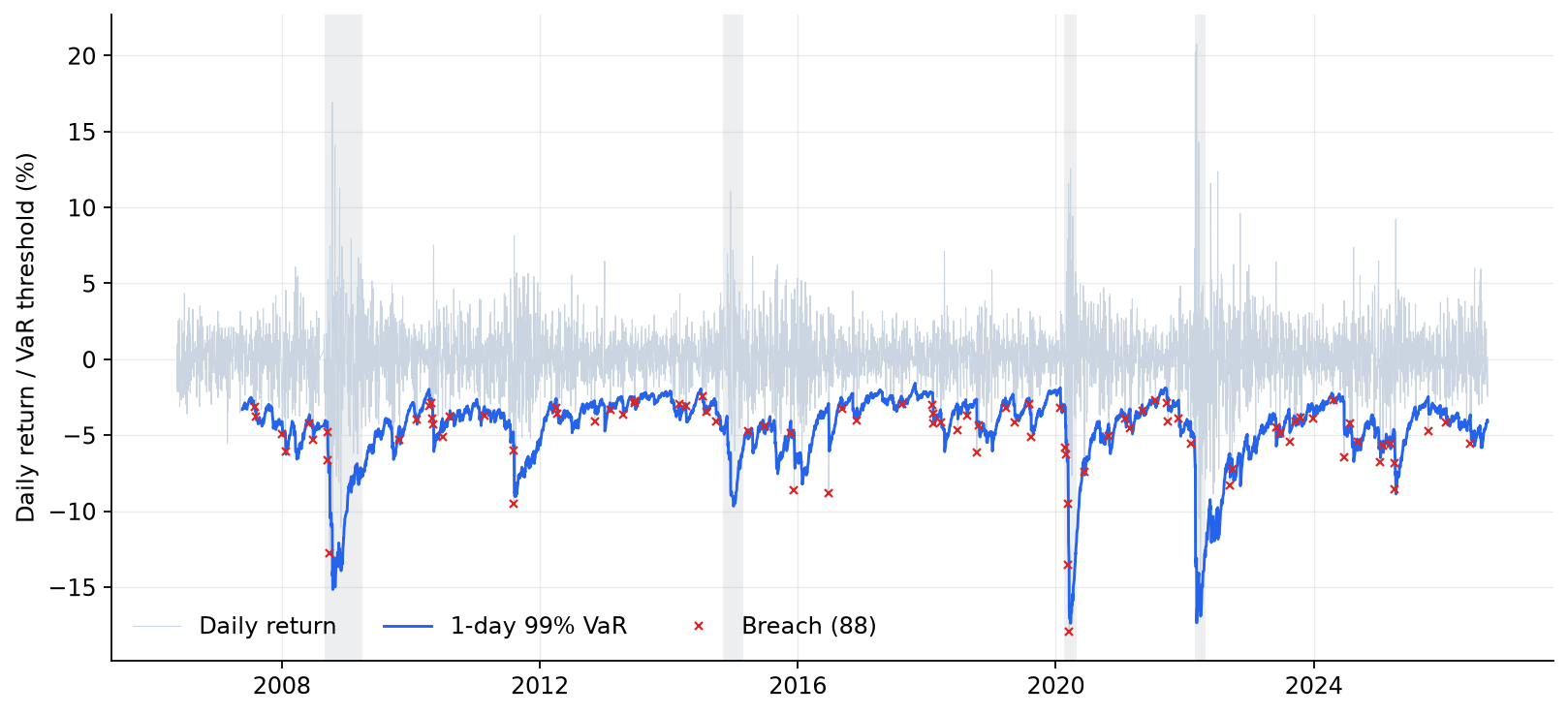
A breach is a day where the realised loss exceeded the forecast. Over 4,738 tested days:

Confidence	Breaches expected	Breaches observed
95%	5.00%	5.21%	well calibrated
99%	1.00%	1.86%	~2× too many
99.9%	0.10%	0.59%	~6× too many

The normal assumption degrades the further into the tail you push it. At 95% the model is essentially right. At 99% it breaches nearly twice as often as advertised, and at 99.9% almost six times as often — a portfolio manager relying on the deep-tail number would be materially under-reserved.

This is the fat-tails problem made concrete. The return distribution shown above has more mass far from the mean than a normal distribution does, and parametric VaR prices that mass at zero. It also explains the ordering in the VaR comparison: historical simulation, which reads the tail off what actually happened rather than assuming a shape, produces the largest and most conservative estimate of the three.

Why this matters more than the point estimate

A VaR figure with no backtest is an assertion. The Basel framework requires banks to backtest exactly this way and penalises models that breach too often - so the interesting output here is not "4.11%", it is "4.11%, and here is how often that class of estimate has been wrong."

Component risk

Setting the exposure vector to isolate each factor:

Exposure	1-day 99% VaR
Equity only	2.90%
Forex only	2.59%
Combined	4.11%
Sum of stand-alone	5.49%
Diversification benefit	1.38%

The combined figure is 1.38 percentage points below the sum of the parts. That gap is the diversification benefit, and it exists because the two risks are not perfectly correlated — the same instability shown in the correlation chart above, now expressed in units of risk.