Quantile Compass¶

Value-at-Risk for a portfolio that carries two different kinds of risk at once.

A ruble-based investor holds a 60/40 portfolio of US (NASDAQ 100) and German (DAX) equities. Because those holdings are priced in dollars and euros, the investor is exposed both to the equity markets and to the currency they are quoted in — and those two exposures do not behave the same way in a crisis.

This project decomposes the portfolio's ruble return into an equity component and a currency component, tracks the volatility and correlation of each through time, and compares three different ways of answering the same question: how much could this portfolio lose tomorrow?

The sample¶


Period	May 2006 – September 2026
Observations	4,988 daily returns
Risk factors	NASDAQ 100, DAX, USD/RUB, EUR/RUB
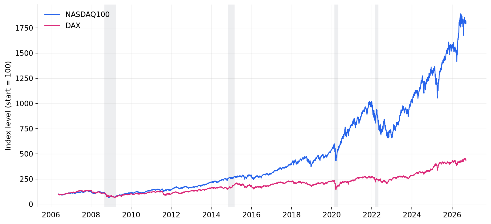
Crises covered	2008 financial crisis · 2014 ruble crisis · COVID-19 · 2022 Russia-Ukraine

Twenty years of daily data spanning four distinct crises — two driven by global equity markets, two specific to the ruble. That contrast is what makes the decomposition worth doing.

Equity indices rebased to 100

What the analysis shows¶

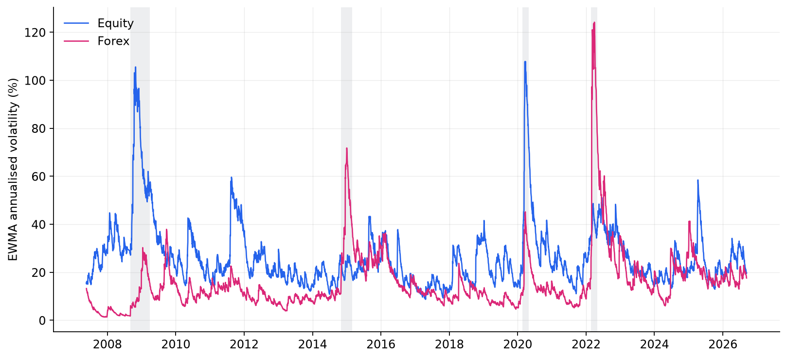
The two risks peak in different crises. Equity volatility peaks in 2008 (≈105% annualised) and again in the COVID crash (107.8% on 19 March 2020). Currency volatility is comparatively quiet through both, then dominates in the 2014 ruble crisis and again in 2022, reaching 124.2% on 31 March 2022 — higher than equity volatility ever gets in this sample.

EWMA annualised volatility

Their correlation is unstable and often negative. Averaging −0.06 over the full sample but ranging from −0.70 to +0.50, the relationship between equity and currency returns is not something you can treat as a constant. When it is negative, a depreciating ruble cushions equity losses for this investor — a natural hedge that appears exactly when it is most useful, and disappears at other times.

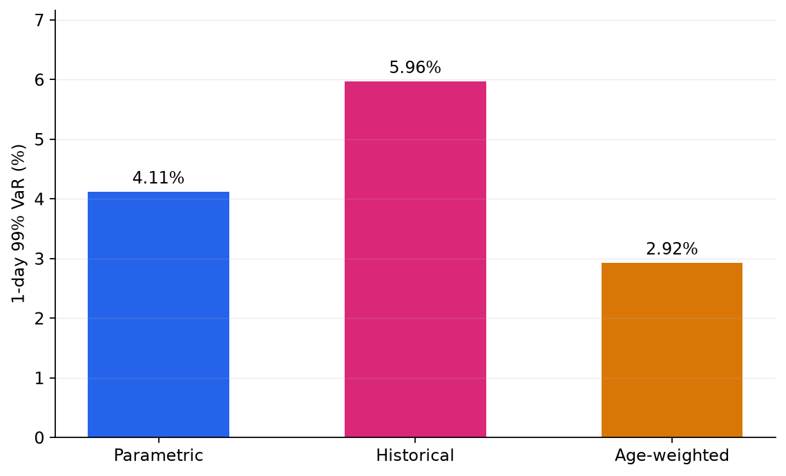
The three VaR methods disagree, and the disagreement is the point. At 99% confidence over one day: parametric gives 4.11%, historical 5.96%, age-weighted 2.92%. Same portfolio, same data, same confidence level — a spread of more than 3 percentage points depending purely on how you weight history.

VaR by method

Try it¶

Open the live app :material-open-in-new:

Change the confidence level, the EWMA decay or the portfolio weights and watch the estimates move.

Getting started¶

git clone https://github.com/omarja12/quantile-compass.git
cd quantile-compass
pip install -e ".[app,dev]"

# the app fetches the dataset itself on first run
streamlit run app/streamlit_app.py

See Methodology for the formulas, Results for the full set of findings, and the API reference for the code.